Zonal Averaging#
This section demonstrates how to perform Zonal Averaging using UXarray, covering both non-conservative and conservative methods.
Notebook Roadmap#
1. Zonal Mean Basics — terminology and the two averaging flavors available in UXarray.
2. Non-Conservative Zonal Averaging — default sampling, intersection-weighted averaging,plotting, and tuning latitude spacing.
3. Conservative Zonal Averaging — area-weighted bands, conservation checks, and comparisons.
4. Combined Plots — pair global maps with their zonal means for context.
5. HEALPix Zonal Averaging (Conservative vs Non-Conservative) — run the same workflow on a different grid.
6. 2D Zonal Means on NE30 (RELHUM) — build latitude–height slices and inspect the differences.
from pathlib import Path

import hvplot.pandas  # noqa: F401 - activate pandas hvplot accessor
import hvplot.xarray  # noqa: F401 - activate xarray hvplot accessor
import matplotlib.pyplot as plt
import numpy as np
import xarray as xr

import uxarray as ux

uxds = ux.open_dataset(
    "../../test/meshfiles/ugrid/outCSne30/outCSne30.ug",
    "../../test/meshfiles/ugrid/outCSne30/outCSne30_vortex.nc",
)
1. Zonal Mean Basics#
Step 1.1: Understand the two averaging flavors#
A zonal average (or zonal mean) is a statistical measure that represents the average of a face-centered variable along lines of constant latitude or over latitudinal bands.
UXarray provides two types of zonal averaging:
Non-conservative: Calculates the mean by sampling face values at specific latitude lines and weighting each contribution by the length of the line where each face intersects that latitude.
Conservative: Preserves integral quantities by calculating the mean by sampling face values within latitude bands and weighting contributions by their area overlap with latitude bands.
See also
NCL Zonal Average — NCL reference with conventional rectilinear grids.
2. Non-Conservative Zonal Averaging#
The non-conservative method samples face values at specific lines of constant latitude and weights each contribution by the length of the intersection between the face and that latitude. This is the default behavior and is suitable for visualization and general analysis where exact conservation is not required.
Step 2.1: Visualize the global field#
The non-conservative method samples face values at specific lines of constant latitude and calculates the average using intersection-line weights. Let’s first visualize our data field and then demonstrate zonal averaging:
# Display the global field
uxds["psi"].plot(cmap="inferno", periodic_elements="split", title="Global Field")
Step 2.2: Compute the default zonal mean#
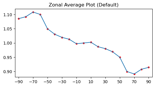
Calling .zonal_mean() with no arguments samples every 10° between -90° and 90° and returns one value per latitude line.
zonal_mean_psi = uxds["psi"].zonal_mean()
zonal_mean_psi
<xarray.DataArray 'psi_zonal_mean' (latitudes: 19)> Size: 152B
array([1.08546247, 1.09219987, 1.10863654, 1.10011333, 1.04989243,
       1.03074397, 1.01980815, 1.01312147, 0.9973705 , 1.00000001,
       1.00262952, 0.98687854, 0.98019186, 0.96925608, 0.95010754,
       0.89988665, 0.89136345, 0.90780013, 0.91453753])
Coordinates:
  * latitudes  (latitudes) float64 152B -90.0 -80.0 -70.0 ... 70.0 80.0 90.0
Attributes:
    zonal_mean:    True
conservative: FalseStep 2.3: Inspect the default sampling#
The default latitude range is between -90 and 90 degrees with a step size of 10 degrees. The plot below shows the resulting profile so you can see how many points are sampled across the globe. The next cell prints the sampled latitude coordinates so you can confirm the 10-degree spacing before looking at the plot.
# Inspect default latitude samples
default_lats = zonal_mean_psi.coords["latitudes"].values
print("Default sample latitudes (10-degree spacing):")
print(f"({', '.join(f'{lat:.0f}' for lat in default_lats)}) deg latitude")
Default sample latitudes (10-degree spacing):
(-90, -80, -70, -60, -50, -40, -30, -20, -10, 0, 10, 20, 30, 40, 50, 60, 70, 80, 90) deg latitude
lats = zonal_mean_psi["latitudes"].values
vals = zonal_mean_psi.values
fig, ax = plt.subplots(figsize=(6, 3))
ax.plot(lats, vals, "-")
ax.scatter(lats, vals, s=12, color="red")
ax.set_title("Zonal Average Plot (Default)")
ax.set_xlim(-95, 95)
ax.set_xticks(np.arange(-90, 100, 20))
plt.show()
Step 2.4: Customize the lat parameter#
The range of latitudes can be modified by using the lat parameter. It accepts:
Single scalar: e.g.,
lat=45List/array: e.g.,
lat=[10, 20]orlat=np.array([10, 20])Tuple: e.g.,
(min_lat, max_lat, step)
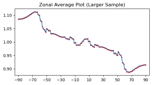
zonal_mean_psi_large = uxds["psi"].zonal_mean(lat=(-90, 90, 1))
Step 2.5: Visualize the higher-resolution sampling#
A 1° step resolves more structure, so the plot below uses the denser coordinate returned from the customized call.
lats = zonal_mean_psi_large["latitudes"].values
vals = zonal_mean_psi_large.values
fig, ax = plt.subplots(figsize=(6, 3))
ax.plot(lats, vals, "-")
ax.scatter(lats, vals, s=4, color="red")
ax.set_title("Zonal Average Plot (Larger Sample)")
ax.set_xlim(-95, 95)
ax.set_xticks(np.arange(-90, 100, 20))
plt.show()
3. Conservative Zonal Averaging#
Conservative zonal averaging preserves integral quantities (mass, energy, momentum) by computing area-weighted averages over latitude bands. This is essential for climate model analysis, energy budget calculations, and any application requiring physical conservation.
Key differences from non-conservative sampling:
Non-conservative: Samples at specific latitude lines
Conservative: Averages over latitude bands between adjacent lines
Conservation: Preserves global integrals to machine precision
Step 3.1: Configure latitude bands and compute the zonal mean#
We pass latitude band edges to .zonal_mean(..., conservative=True) so each band carries the correct area weight.
# Conservative zonal averaging with bands
bands = np.array([-90, -60, -30, 0, 30, 60, 90])
conservative_result = uxds["psi"].zonal_mean(lat=bands, conservative=True)
conservative_result
<xarray.DataArray 'psi_zonal_mean' (latitudes: 6)> Size: 48B
array([1.10364701, 1.03903852, 1.00581915, 0.9937623 , 0.96140404,
       0.89634629])
Coordinates:
  * latitudes  (latitudes) float64 48B -75.0 -45.0 -15.0 15.0 45.0 75.0
Attributes:
    zonal_mean:      True
    conservative:    True
lat_band_edges: [-90. -60. -30. 0. 30. 60. 90.]Step 3.2: Verify conservation#
A key advantage of conservative zonal averaging is that it preserves global integrals.
# Test conservation property
global_mean = uxds["psi"].mean()
full_sphere_conservative = uxds["psi"].zonal_mean(lat=[-90, 90], conservative=True)
conservation_error = abs(global_mean.values - full_sphere_conservative.values[0])

print(f"Global mean: {global_mean.values:.12f}")
print(f"Conservative full sphere: {full_sphere_conservative.values[0]:.12f}")
print(f"Conservation error: {conservation_error:.2e}")
Global mean: 1.000000001533
Conservative full sphere: 1.000000001829
Conservation error: 2.96e-10
Step 3.3: Understand the lat parameter signature#
Both conservative and non-conservative modes can use the same lat parameter, but they interpret it differently:
Non-conservative: Creates sample points at the specified latitudes
Conservative: Uses the latitudes as band edges, creating bands between adjacent points
# Demonstrate signature behavior
lat_tuple = (-90, 90, 30)  # Every 30 degrees

# Non-conservative: samples at lines
non_cons_lines = uxds["psi"].zonal_mean(lat=lat_tuple)
print(f"Non-conservative with lat={lat_tuple}:")
print(f"Sample points: {non_cons_lines.coords['latitudes'].values}")
print(f"Count: {len(non_cons_lines.coords['latitudes'].values)} points")

# Conservative: creates bands between lines
cons_bands = uxds["psi"].zonal_mean(lat=lat_tuple, conservative=True)
print(f"\nConservative with lat={lat_tuple}:")
print(f"Band centers: {cons_bands.coords['latitudes'].values}")
print(f"Count: {len(cons_bands.coords['latitudes'].values)} bands")
Non-conservative with lat=(-90, 90, 30):
Sample points: [-90. -60. -30.   0.  30.  60.  90.]
Count: 7 points

Conservative with lat=(-90, 90, 30):
Band centers: [-75. -45. -15.  15.  45.  75.]
Count: 6 bands
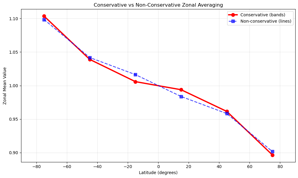
Step 3.4: Visual comparison (lines vs bands)#
The differences between methods reflect their fundamental approaches:
Conservative: More accurate for physical quantities because it accounts for the actual area of each face within latitude bands
Non-conservative: Faster but approximates by sampling at specific latitude lines
The differences you see indicate how much area-weighting matters for your specific data and grid resolution.
# Compare with non-conservative at same latitudes
band_centers = 0.5 * (bands[:-1] + bands[1:])
non_conservative_comparison = uxds["psi"].zonal_mean(lat=band_centers)

# Create comparison plot
fig, ax = plt.subplots(1, 1, figsize=(10, 6))

ax.plot(
    conservative_result.coords["latitudes"],
    conservative_result.values,
    "o-",
    label="Conservative (bands)",
    linewidth=3,
    markersize=8,
    color="red",
)
ax.plot(
    non_conservative_comparison.coords["latitudes"],
    non_conservative_comparison.values,
    "s--",
    label="Non-conservative (lines)",
    linewidth=2,
    markersize=7,
    color="blue",
    alpha=0.7,
)

ax.set_xlabel("Latitude (degrees)")
ax.set_ylabel("Zonal Mean Value")
ax.set_title("Conservative vs Non-Conservative Zonal Averaging")
ax.grid(True, alpha=0.3)
ax.legend()
ax.set_xlim(-90, 90)

plt.tight_layout()
plt.show()
Step 3.5: Quantify the differences#
The differences between conservative and non-conservative results depend on several factors:
Grid Resolution: Higher resolution grids show smaller differences
Data Variability: Rapidly changing fields show larger differences
Latitude Band Size: Wider bands increase the importance of area-weighting
Which is more accurate?
Conservative: More accurate for physical quantities (mass, energy, momentum) because it preserves integral properties
Non-conservative: Adequate for visualization and qualitative analysis
When differences matter most:
Variable resolution grids (where face sizes vary significantly)
Physical conservation requirements
Quantitative analysis and budget calculations
# Quantify the differences
differences = conservative_result.values - non_conservative_comparison.values
max_diff = np.max(np.abs(differences))
mean_diff = np.mean(np.abs(differences))

print(f"Maximum absolute difference: {max_diff:.6f}")
print(f"Mean absolute difference: {mean_diff:.6f}")
print(
    f"Relative difference (max): {max_diff / np.mean(np.abs(conservative_result.values)) * 100:.3f}%"
)
Maximum absolute difference: 0.010503
Mean absolute difference: 0.006114
Relative difference (max): 1.050%
4. Combined Plots#
Step 4.1: Pair a global map with its zonal mean#
It is often desired to plot the zonal average alongside other plots, such as color or contour plots, so you can see both the spatial distribution and its latitude summary in one glance.
# Pair the map and the zonal profile using hvplot
zonal_df = zonal_mean_psi.to_dataframe(name="zonal_mean").reset_index()
map_panel = (
    uxds["psi"]
    .plot(cmap="inferno", periodic_elements="split")
    .opts(title="Global Field", colorbar=True, width=525, height=400)
)
profile_line = zonal_df.hvplot(
    x="zonal_mean",
    y="latitudes",
    line_width=2,
    xlabel="Zonal Mean Value",
    ylabel="Latitude (degrees)",
    title="Latitude Profile",
    ylim=(-90, 90),
    width=400,
    height=400,
)
profile_points = zonal_df.hvplot.scatter(
    x="zonal_mean",
    y="latitudes",
    color="blue",
    size=6,
)
profile_panel = (profile_line * profile_points).opts(show_grid=True)
(map_panel + profile_panel).cols(2)
5. HEALPix Zonal Averaging (Conservative vs Non-Conservative)#
Step 5.1: Compare conservative and non-conservative averages on HEALPix#
This example demonstrates the key differences between conservative (area-weighted) and non-conservative (point-sampling) zonal averaging on a HEALPix grid.
# HEALPix Zonal Averaging: Conservative vs Non-Conservative Methods
# This example demonstrates the key differences between conservative (area-weighted)
# and non-conservative (point-sampling) zonal averaging on a HEALPix grid.
# Create HEALPix grid with synthetic data
# Using sin(latitude) as test function - varies smoothly with latitude
uxgrid = ux.Grid.from_healpix(zoom=3, pixels_only=False)
data = np.sin(np.deg2rad(uxgrid.face_lat.values))
uxda = ux.UxDataArray(data, uxgrid=uxgrid, dims=["n_face"], name="val")

# Define analysis region: 20° latitude band centered at 42°N
band_edges = np.array([32.0, 52.0])  # Southern USA to Canada
lat_center = 42.0  # Approximate latitude of Chicago/Boston

# Method 1: Conservative zonal mean (area-weighted average over band)
# - Integrates data over entire latitude band
# - Accounts for spherical geometry (smaller areas near poles)
# - Preserves physical quantities like total energy/mass
z_cons = uxda.zonal_mean(lat=band_edges, conservative=True)

# Method 2: Non-conservative zonal mean (point sampling at specific latitude)
# - Samples data at exact latitude circle
# - Faster computation, simpler interpretation
# - Better for comparison with station observations
z_noncons = uxda.zonal_mean(lat=lat_center)

# Calculate theoretical values for validation
theoretical_point = np.sin(np.deg2rad(lat_center))  # Exact at 42°N
# For band average: integrate sin(lat)*cos(lat) / integrate cos(lat)
lat_s, lat_n = np.deg2rad(band_edges)
theoretical_band = (
    0.5 * (np.sin(lat_n) ** 2 - np.sin(lat_s) ** 2) / (np.sin(lat_n) - np.sin(lat_s))
)

# Display results
print("=" * 65)
print("ZONAL AVERAGING ON HEALPix GRID: Conservative vs Non-Conservative")
print("=" * 65)
print("\nTest function: sin(latitude)")
print(f"Analysis band: {band_edges[0]:.0f}°N to {band_edges[1]:.0f}°N")
print(f"Center latitude: {lat_center:.0f}°N")
print("Grid resolution: HEALPix zoom level 3 (~1.8° spacing)")

print("\n" + "-" * 65)
print("RESULTS:")
print("-" * 65)
print(f"Conservative (band average):     {float(z_cons.values[0]):.4f}")
print(f"  → Theoretical value:            {theoretical_band:.4f}")
print("  → Physical meaning: Area-weighted average over 20° band")
print("  → Use case: Flux calculations, energy budgets\n")

print(f"Non-conservative (point value):  {float(z_noncons.values[0]):.4f}")
print(f"  → Theoretical value:            {theoretical_point:.4f}")
print(f"  → Physical meaning: Value at exactly {lat_center}°N")
print("  → Use case: Station comparisons, spot measurements")

print("\n" + "-" * 65)
print("KEY INSIGHTS:")
print("-" * 65)
difference = float(z_noncons.values[0]) - float(z_cons.values[0])
print(
    f"• Difference between methods: {difference:.4f} ({difference / float(z_noncons.values[0]) * 100:.1f}%)"
)
print("• Conservative < Non-conservative because sin(lat) increases toward")
print("  the pole, and southern portion of band has lower values")
print("• Both methods are 'correct' - choose based on your application:")
print("  - Conservative: preserves integrated quantities")
print("  - Non-conservative: provides local values")
=================================================================
ZONAL AVERAGING ON HEALPix GRID: Conservative vs Non-Conservative
=================================================================

Test function: sin(latitude)
Analysis band: 32°N to 52°N
Center latitude: 42°N
Grid resolution: HEALPix zoom level 3 (~1.8° spacing)

-----------------------------------------------------------------
RESULTS:
-----------------------------------------------------------------
Conservative (band average):     0.6528
  → Theoretical value:            0.6590
  → Physical meaning: Area-weighted average over 20° band
  → Use case: Flux calculations, energy budgets

Non-conservative (point value):  0.6687
  → Theoretical value:            0.6691
  → Physical meaning: Value at exactly 42.0°N
  → Use case: Station comparisons, spot measurements

-----------------------------------------------------------------
KEY INSIGHTS:
-----------------------------------------------------------------
• Difference between methods: 0.0159 (2.4%)
• Conservative < Non-conservative because sin(lat) increases toward
  the pole, and southern portion of band has lower values
• Both methods are 'correct' - choose based on your application:
  - Conservative: preserves integrated quantities
  - Non-conservative: provides local values
6. 2D Zonal Means on NE30 (RELHUM)#
Everything above uses a single-level field. For the NE30 multi-level RELHUM data, we can see how a zonal mean collapses every longitude in each latitude ring—averaging the native face values with intersection-line (non-conservative) or area (conservative) weights—so the result becomes a latitude–height diagnostic, unlike a cross section that interpolates to create a 2D output over a single path. Each step below walks through the process with extra explanations for first-time users.
Tip
zonal_mean() works directly on the native cell values to build latitude-only diagnostics. When you instead need interpolation along a specified great-circle or constant-lon/lat path, use .cross_section() to construct that transect and see the Cross-Sections guide for path-based examples.
Step 6.1: Load the NE30 grid and prepare the field#
We point UXarray to the grid and data files under test/meshfiles/scrip/ne30pg2/, open the RELHUM variable, and drop the leading time dimension so the array is only (level, face).
grid_path = Path("../../test/meshfiles/scrip/ne30pg2/grid.nc")
data_path = Path("../../test/meshfiles/scrip/ne30pg2/data.nc")

ne30_ds = ux.open_dataset(grid_path, data_path)
relhum = ne30_ds["RELHUM"]

for dim in ("time", "t", "step"):
    if dim in relhum.dims:
        relhum = relhum.isel({dim: 0})

level_dim = "level" if "level" in relhum.dims else relhum.dims[0]
levels = relhum.coords.get(
    level_dim,
    xr.DataArray(np.arange(relhum.sizes[level_dim]), dims=level_dim),
).values

relhum
<xarray.UxDataArray 'RELHUM' (lev: 72, n_face: 21600)> Size: 6MB
[1555200 values with dtype=float32]
Coordinates:
  * lev      (lev) float64 576B 0.1238 0.1828 0.2699 ... 986.2 993.8 998.5
    time     object 8B ...
Dimensions without coordinates: n_face
Attributes:
    mdims:          1
    units:          percent
    long_name:      Relative humidity
    standard_name:  relative_humidity
cell_methods: time: meanStep 6.2: Build latitude samples and compute both zonal means#
Sampling every 10 degrees gives us clearly separated latitude bands while staying light on compute. The non-conservative average uses those values as centers, while the conservative option treats them as band edges so that each band carries the correct area weight. Adjust the spacing if you need higher detail or faster turnaround.
lat_edges_deg = np.arange(-90.0, 90.0 + 10.0, 10.0)
lat_centers_deg = 0.5 * (lat_edges_deg[:-1] + lat_edges_deg[1:])


def stack_zonal_means(data_array, lat_values, *, conservative):
    slices = []
    for lev in range(data_array.sizes[level_dim]):
        zonal_slice = data_array.isel({level_dim: lev}).zonal_mean(
            lat=lat_values, conservative=conservative
        )
        slices.append(zonal_slice)
    zonal = xr.concat(slices, dim=level_dim)
    return zonal.assign_coords({level_dim: levels}).rename({"latitudes": "lat"})


zonal_nc = stack_zonal_means(relhum, lat_centers_deg, conservative=False)
zonal_c = stack_zonal_means(relhum, lat_edges_deg, conservative=True)
zonal_diff = zonal_c - zonal_nc

zonal_nc
<xarray.DataArray 'RELHUM_zonal_mean' (lev: 72, lat: 18)> Size: 5kB
array([[1.39507087e-04, 1.46236242e-04, 1.57333357e-04, ...,
        1.38013987e-04, 1.37959549e-04, 1.37912750e-04],
       [1.46500082e-04, 1.56465467e-04, 1.59396877e-04, ...,
        1.38380448e-04, 1.37978277e-04, 1.37925847e-04],
       [1.39333293e-04, 1.40268996e-04, 1.41239536e-04, ...,
        1.41590019e-04, 1.37986484e-04, 1.37942334e-04],
       ...,
       [9.95636673e+01, 9.57479248e+01, 9.42285156e+01, ...,
        1.00770416e+02, 1.01268219e+02, 1.04364807e+02],
       [9.75083466e+01, 9.47997131e+01, 9.26638336e+01, ...,
        9.82491531e+01, 9.99979477e+01, 1.02430000e+02],
       [9.58398132e+01, 9.40848160e+01, 9.15409851e+01, ...,
        9.66513596e+01, 9.93786469e+01, 1.01074776e+02]],
      shape=(72, 18), dtype=float32)
Coordinates:
  * lev      (lev) float64 576B 0.1238 0.1828 0.2699 ... 986.2 993.8 998.5
  * lat      (lat) float64 144B -85.0 -75.0 -65.0 -55.0 ... 55.0 65.0 75.0 85.0
Attributes:
    zonal_mean:    True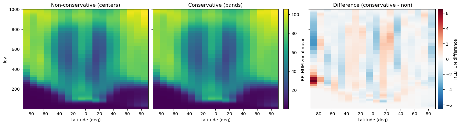
conservative: FalseStep 6.3: Visualize the latitude–level slices#
Placing the two 2D sections next to each other shows the smoothing introduced by area weighting, while a third panel plotting the signed difference (conservative − non-conservative) highlights where the methods diverge. Because every panel uses the same color scale (and the difference plot uses a diverging palette), the contrast is easy to spot.
fig, axes = plt.subplots(1, 3, figsize=(15, 4), sharey=True, constrained_layout=True)

value_min = float(min(zonal_nc.min().values, zonal_c.min().values))
value_max = float(max(zonal_nc.max().values, zonal_c.max().values))

mesh_nc = axes[0].pcolormesh(
    zonal_nc["lat"],
    levels,
    zonal_nc.transpose(level_dim, "lat"),
    shading="nearest",
    cmap="viridis",
    vmin=value_min,
    vmax=value_max,
)
axes[0].set_title("Non-conservative (centers)")
axes[0].set_xlabel("Latitude (deg)")
axes[0].set_ylabel(level_dim)
axes[0].set_xlim(-90, 90)

mesh_c = axes[1].pcolormesh(
    zonal_c["lat"],
    levels,
    zonal_c.transpose(level_dim, "lat"),
    shading="nearest",
    cmap="viridis",
    vmin=value_min,
    vmax=value_max,
)
axes[1].set_title("Conservative (bands)")
axes[1].set_xlabel("Latitude (deg)")
axes[1].set_xlim(-90, 90)

diff_max = float(np.nanmax(np.abs(zonal_diff.values)))
if diff_max == 0:
    diff_max = 1e-6
mesh_diff = axes[2].pcolormesh(
    zonal_diff["lat"],
    levels,
    zonal_diff.transpose(level_dim, "lat"),
    shading="nearest",
    cmap="RdBu_r",
    vmin=-diff_max,
    vmax=diff_max,
)
axes[2].set_title("Difference (conservative - non)")
axes[2].set_xlabel("Latitude (deg)")
axes[2].set_xlim(-90, 90)

cbar_field = fig.colorbar(
    mesh_nc, ax=[axes[0], axes[1]], orientation="vertical", fraction=0.04, pad=0.02
)
cbar_field.set_label("RELHUM zonal mean")

cbar_diff = fig.colorbar(
    mesh_diff, ax=[axes[2]], orientation="vertical", fraction=0.08, pad=0.02
)
cbar_diff.set_label("RELHUM difference")
Step 6.4: Spot-check the difference numerically#
Visuals are helpful, but printing quick summary statistics and a few sample latitude bands makes it clear how large the conservative correction is.
abs_diff = np.abs(zonal_diff)
max_abs = float(abs_diff.max())
mean_abs = float(abs_diff.mean())
per_level_max = abs_diff.max(dim="lat")

print(f"Max absolute difference: {max_abs:.3f}")
print(f"Mean absolute difference: {mean_abs:.3f}")

preview_levels = per_level_max.isel({level_dim: slice(0, 5)})
preview_levels
Max absolute difference: 6.528
Mean absolute difference: 0.488
<xarray.DataArray 'RELHUM_zonal_mean' (lev: 5)> Size: 20B
array([2.2769236e-06, 3.7543796e-06, 2.1681481e-06, 4.8164511e-06,
       2.9183575e-06], dtype=float32)
Coordinates:
  * lev      (lev) float64 40B 0.1238 0.1828 0.2699 0.3986 0.5885
Attributes:
    zonal_mean:      True
    lat_band_edges:  [-90. -80. -70. -60. -50. -40. -30. -20. -10.   0.  10. ...