Compatibility with HoloViz Tools

This user guide section showcases how UXarray data structures (Grid, UxDataArray) can be converted in a Spatialpandas GeoDataFrame, which can be used directly by packages from the HoloViz stack, such as hvPlot, Datashader, Holoviews, and Geoviews. In addition to showing how to convert to a GeoDataFrame, a series of visualizations using hvPlot and GeoViews is showcased based around the converted data structure.

import warnings

import holoviews as hv
import hvplot.pandas
import matplotlib
import matplotlib.pyplot as plt
import numpy as np

import uxarray as ux

warnings.filterwarnings("ignore")

Data

For this notebook, we will be using E3SM model output, which uses a cubed-sphere grid. However, this notebook can be adapted to datasets in any of our supported formats.

base_path = "../../test/meshfiles/ugrid/outCSne30/"
grid_path = base_path + "outCSne30.ug"
data_path = base_path + "outCSne30_vortex.nc"

uxds = ux.open_dataset(grid_path, data_path)

uxds

<xarray.UxDataset> Size: 43kB
Dimensions:  (n_face: 5400)
Dimensions without coordinates: n_face
Data variables:
    psi      (n_face) float64 43kB ...

<xarray.UxDataset> Size: 43kB
Dimensions:  (n_face: 5400)
Dimensions without coordinates: n_face
Data variables:
    psi      (n_face) float64 43kB ...

uxarray.UxDataset

• Dimensions:
  • n_face: 5400
• Coordinates: (0)
• Data variables: (1)
  • psi
    (n_face)
    float64
    ...

    [5400 values with dtype=float64]

• Indexes: (0)
• Attributes: (0)

Show Grid Information

<uxarray.Grid>
Original Grid Type: UGRID
Grid Dimensions:
  * n_node: 5402
  * n_face: 5400
  * n_max_face_nodes: 4
Grid Coordinates (Spherical):
  * node_lon: (5402,)
  * node_lat: (5402,)
Grid Coordinates (Cartesian):
Grid Connectivity Variables:
  * face_node_connectivity: (5400, 4)
Grid Descriptor Variables:

uxarray.UxDataset.uxgrid

• Dimensions:
  • n_face: 5400
  • n_max_face_nodes: 4
  • n_node: 5402
• Spherical Coordinates: (2)
  • node_lon
    (n_node)
    float64
    -45.0 45.0 135.0 ... 138.0 135.0

    standard_name :

    longitude

    long_name :

    longitude of 2D mesh nodes

    units :

    degrees_east

    array([-45.        ,  45.        , 135.        , ..., 141.09968961,
           138.03317102, 135.        ], shape=(5402,))

  • node_lat
    (n_node)
    float64
    ...

    standard_name :

    latitude

    long_name :

    latitude of 2D mesh nodes

    units :

    degrees_north

    [5402 values with dtype=float64]

• Cartesian Coordinates: (0)
• Connectivity: (1)
  • face_node_connectivity
    (n_face, n_max_face_nodes)
    int64
    0 8 356 124 8 ... 5401 297 6 298

    cf_role :

    face_node_connectivity

    start_index :

    0

    _FillValue :

    -9223372036854775808

    array([[   0,    8,  356,  124],
           [   8,    9,  357,  356],
           [   9,   10,  358,  357],
           ...,
           [5399, 5400,  299,  300],
           [5400, 5401,  298,  299],
           [5401,  297,    6,  298]], shape=(5400, 4))

• Descriptors: (0)
• Attributes: (1)

  source_grid_spec :

  UGRID

Conversion to spatialpandas.GeoDataFrame for Visualization

In order to support visualization with the popular HoloViz stack of libraries (hvPlot, HoloViews, Datashader, etc.), UXarray provides methods for converting Grid and UxDataArray objects into a SpatialPandas GeoDataFrame, which can be used for visualizing the nodes, edges, and polygons that represent each grid, in addition to data variables.

Grid Conversion

If you wish to plot only the grid’s geometrical elements such as nodes and edges (i.e. without any data variables mapped to them), you can directly convert a Grid instance into a GeoDataFrame.

Each UxDataset and UxDataArray has a Grid instance paired to it, which can be accessed using the .uxgrid attribute.

You can use the Grid.to_geodataframe() method to construct a GeoDataFrame.

gdf_grid = uxds.uxgrid.to_geodataframe()
gdf_grid

	geometry
0	Polygon([[-45.0, -35.26438903808594, -42.0, -3...
1	Polygon([[-42.0, -36.61769485473633, -39.0, -3...
2	Polygon([[-39.0, -37.852420806884766, -36.0, -...
3	Polygon([[-36.0, -38.973445892333984, -33.0, -...
4	Polygon([[-33.0, -39.98556900024414, -30.0, -4...
...	...
5333	Polygon([[147.3314971923828, 43.07368087768555...
5334	Polygon([[144.1993408203125, 42.01158142089844...
5335	Polygon([[141.0996856689453, 40.83760452270508...
5336	Polygon([[138.03317260742188, 39.5490798950195...
5337	Polygon([[135.0, 38.143314361572266, 132.0, 36...

5338 rows × 1 columns

UxDataArray & UxDataset Conversion

If you are interested in mapping data to each face, you can index the UxDataset with the variable of interest (in this case “psi”) to return the same GeoDataFrame as above, but now with data mapped to each face.

Warning

UXarray currently only supports mapping data variables that are mapped to each face. Variables that reside on the corner nodes or edges are currently not supported for visualization.

gdf_data = uxds["psi"].to_geodataframe()
gdf_data

	geometry	psi
0	Polygon([[-45.0, -35.26438903808594, -42.0, -3...	1.351317
1	Polygon([[-42.0, -36.61769485473633, -39.0, -3...	1.330915
2	Polygon([[-39.0, -37.852420806884766, -36.0, -...	1.310140
3	Polygon([[-36.0, -38.973445892333984, -33.0, -...	1.289056
4	Polygon([[-33.0, -39.98556900024414, -30.0, -4...	1.267717
...	...	...
5333	Polygon([[147.3314971923828, 43.07368087768555...	0.733539
5334	Polygon([[144.1993408203125, 42.01158142089844...	0.712085
5335	Polygon([[141.0996856689453, 40.83760452270508...	0.690883
5336	Polygon([[138.03317260742188, 39.5490798950195...	0.669989
5337	Polygon([[135.0, 38.143314361572266, 132.0, 36...	0.649467

5338 rows × 2 columns

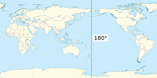
Challenges with Representing Geoscience Data as Geometries

When we convert to a GeoDataFrame, we internally represent the surface of a sphere as a collection of polygons over a 2D projection. However, this leads to issues around the Antimeridian (180 degrees east or west) where polygons are incorrectly constructed and have incorrect geometries. When constructing the GeoDataFrame, UXarray detects and corrects any polygon that touches or crosses the antimeridian. An array of indices of these faces can be accessed as part of the Grid object.

Antimeridian Visual

uxds.uxgrid.antimeridian_face_indices

array([1814, 1844, 1874, 1904, 1934, 1964, 1994, 2024, 2054, 2084, 2114,
       2144, 2174, 2204, 2234, 2264, 2294, 2324, 2354, 2384, 2414, 2444,
       2474, 2504, 2534, 2564, 2594, 2624, 2654, 2684, 3615, 3645, 3675,
       3705, 3735, 3765, 3795, 3825, 3855, 3885, 3915, 3945, 3975, 4005,
       4034, 4035, 4964, 4965, 4995, 5025, 5055, 5085, 5115, 5145, 5175,
       5205, 5235, 5265, 5295, 5325, 5355, 5385])

Taking a look at one of these faces that crosses or touches the antimeridian, we can see that it’s split across the antimeridian and represented as a MultiPolygon, which allows us to properly render this two dimensional grid.

gdf_data.geometry[uxds.uxgrid.antimeridian_face_indices[0]]

Polygon([[-180.0, -45.0, -177.0, -44.96071243286133, -177.0, -41.96092987060547, -180.0, -42.0, -180.0, -45.0]])

For more details about the algorithm used for splitting these polygons, see the Antimeridian Python Package, which we use internally for correcting polygons on the antimeridian.

Visualizing Geometries

The next sections will show how the GeoDataFrame representing our unstructured grid can be used with hvPlot and GeoViews to generate visualizations. Examples using both the matplotlib and bokeh backends are shown, with bokeh examples allowing for interactive plots.

Nodes

# use matplotlib backend for rendering
hv.extension("matplotlib")

plot_kwargs = {
    "size": 6.0,
    "xlabel": "Longitude",
    "ylabel": "Latitude",
    "coastline": True,
    "width": 1600,
    "title": "Node Plot (Matplotlib Backend)",
}


gdf_grid.hvplot.points(**plot_kwargs)

ⓘ

# use bokeh backend for rendering
hv.extension("bokeh")

plot_kwargs = {
    "s": 1.0,
    "xlabel": "Longitude",
    "ylabel": "Latitude",
    "coastline": True,
    "frame_width": 700,
    "title": "Node Plot (Bokeh Backend)",
}

gdf_grid.hvplot.points(**plot_kwargs)

ⓘ

Edges

# use matplotlib backend for rendering
hv.extension("matplotlib")

plot_kwargs = {
    "linewidth": 1.0,
    "xlabel": " Longitude",
    "ylabel": "Latitude",
    "coastline": True,
    "width": 1600,
    "title": "Edge Plot (Matplotlib Backend)",
    "color": "black",
}

import cartopy.crs as ccrs

gdf_grid.hvplot.paths(**plot_kwargs)

ⓘ

# use bokeh backend for rendering
hv.extension("bokeh")

plot_kwargs = {
    "line_width": 0.5,
    "xlabel": "Longitude",
    "ylabel": "Latitude",
    "coastline": True,
    "frame_width": 700,
    "title": "Edge Plot (Bokeh Backend)",
}

gdf_grid.hvplot.paths(**plot_kwargs)

ⓘ

Visualizing Data Variables

hv.extension("matplotlib")

plot_kwargs = {
    "c": "psi",
    "cmap": "inferno",
    "width": 400,
    "height": 200,
    "title": "Filled Polygon Plot (Matplotlib Backend, Rasterized)",
    "xlabel": " Longitude",
    "ylabel": "Latitude",
}

gdf_data.hvplot.polygons(**plot_kwargs, rasterize=True)

ⓘ

Note

Visualizing filled polygons without rasterization using the matplotlib backend produces incorrect results, see hvplot/#1099

hv.extension("bokeh")

plot_kwargs = {
    "c": "psi",
    "cmap": "inferno",
    "line_width": 0.1,
    "frame_width": 500,
    "frame_height": 250,
    "xlabel": " Longitude",
    "ylabel": "Latitude",
}

gdf_data.hvplot.polygons(**plot_kwargs, rasterize=True)

hv.Layout(
    gdf_data.hvplot.polygons(**plot_kwargs, rasterize=True).opts(
        title="Filled Polygon Plot (Bokeh Backend, Rasterized)"
    )
    + gdf_data.hvplot.polygons(**plot_kwargs, rasterize=False).opts(
        title="Filled Polygon Plot (Bokeh Backend, Vector)"
    )
).cols(1)

ⓘ

Geographic Projections

hv.extension("matplotlib")

plot_kwargs = {
    "c": "psi",
    "cmap": "inferno",
    "width": 400,
    "height": 200,
    "title": "Filled Polygon Plot (Matplotlib Backend, Rasterized, Orthographic Projection)",
    "xlabel": " Longitude",
    "ylabel": "Latitude",
}

gdf_data.hvplot.polygons(**plot_kwargs, rasterize=True, projection=ccrs.Orthographic())

ⓘ

hv.extension("matplotlib")

plot_kwargs = {
    "c": "psi",
    "cmap": "inferno",
    "width": 400,
    "height": 200,
    "title": "Filled Polygon Plot (Matplotlib Backend, Rasterized, Robinson Projection)",
    "xlabel": " Longitude",
    "ylabel": "Latitude",
}

gdf_data.hvplot.polygons(**plot_kwargs, rasterize=True, projection=ccrs.Robinson())

ⓘ